Photon Shot Noise Explained
By Yiheng Chi and Stanley Chan, DeepLux Technology Inc.
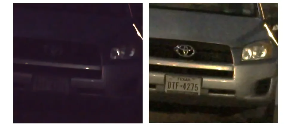
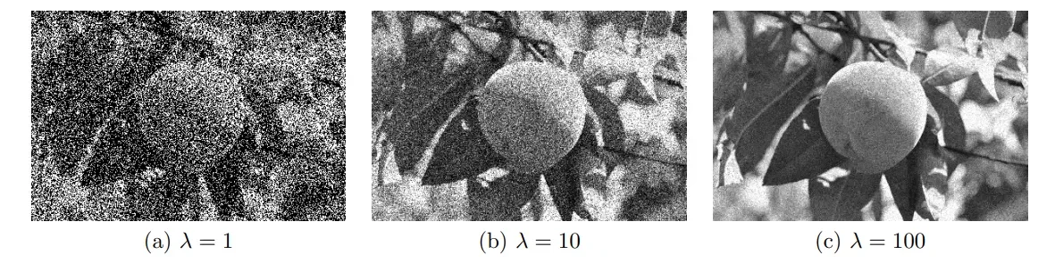
A comment we constantly hear from sensor folks is that the image sensor is the biggest bottleneck in camera today. This roughly implies that if there is a perfect sensor, then we will obtain the true image. But the caveat here is a sensor will never give us the true image. Any image we acquire will still going to be noisy. Yes, we will get a noisy image even if we have a perfect image sensor that has zero defect and 100% quantum efficiency. As long as the exposure is short or the environment is dark, the image will be noisy. (See Figure 1.) This is Mother Nature, and the randomness is photon shot noise.
Figure 1. When photon level decreases, we see more noise. One of the leading reasons for this phenomenon is the random photon arrivals.
Photoevent
But exactly what is photon shot noise? To answer this question we need to first briefly explain the quantum nature of a photon. Unlike a grain of sand or a piece of marble, a photon is not a physical particle but quantized packet of energy. When a photon hits the surface of a material (e.g., silicon), the energy carried by the photon will transferred. If the energy exceeds the bandgap of the material, a photoevent will be triggered. Otherwise the photon energy will just dissipate as heat. A photoevent can be summarized as:
Photoevent = the event in which energy is successfully transferred from a photon to generate mobile electrical charges.
As the conversion from photon energy to electrical charges is a random process, a photoevent is technically a random variable taking a binary state
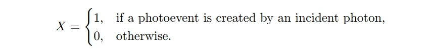
Because it is a random variable, we need to define its probability distribution. But since the random variable X is binary, the probability distribution is Bernoulli:

where η defines the quantum efficiency. Therefore, quantum efficiency is the probability where a photoevent happens. Some people define quantum efficiency as the ratio between number of photoevents and the total number of incident photons. This is also correct, but in an asymptotic sense. If we define a sequence of random variables X₁, X₂, …, Xₙ where each one is a Bernoulli random variable, then the average will give us the sample average which will converge in probability to the true η:

Probability Distribution of K Photoevents
Suppose now we have N incident photons. Because each photoevent is a Bernoulli random variable, the sum of all these N incident photons will give us

Since K is a sum of random variables, itself must also be a random variable. Undergraduate probability textbooks tell us that since each X is Bernoulli, K must be a binomial random variable.

Note that here we condition K on N, because the number of incident photons N is technically random as well. We will talk about its distribution shortly.
Randomness in Number of Incident Photons N
The final piece of puzzle is the number of incident photons N. When photons come off from a source (be it emitted directly from the source or bounced due to reflection), the number N is never a deterministic integer. The modeling of this N can be described by the standard independent increment principle, which states the probability of emitting one photon is linearly proportional to the rate (i.e., the flux), and there is one and only one photon during any short observation interval.
Under these assumptions, we can show that

where λ is the rate of photon arrivals (in the unit of number per seconds). Now substituting this distribution into the conditional distribution of K given N, and by using the law of total probability, we can easily derive
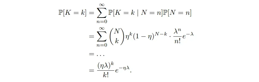
This gives us the glorious Poisson distribution. Therefore, the number of photoevents is distributed according to Poisson. The rate is determined by the quantum efficiency η and the arrival rate λ.
Photon Shot Noise
Now that we understand the model of the photoevents, we can easily understand the nature of photon shot noise. Photon shot noise is nothing but the random fluctuation demonstrated by the random variable K. Our electronic circuits display the number of electrical charges. This is the result of the photoevent.
At different regions of an image, a brighter area will give us a larger λ and hence a larger average K. Similarly, a darker area will give us a smaller average K.
Some people prefers to model the Poisson distribution via a signal dependent Gaussian as follows.

This is generally valid for a large enough λ. The benefit of using a Gaussian is that we can easily define the signal to noise ratio by recognizing the signal and the noise standard deviation. The following is a Python code demonstrating the difference between the Poisson modeling and the Gaussian approximation. Notably, the generation of the Gaussian approximation is much faster. And when λ is large enough, the Gaussian approximation is fairly good.
# Python
# Python Code to demonstrate the speed difference
# when using the Gaussian approximation.
import numpy as np
import time

# Poisson Distribution
start = time.time()
X = np.random.poisson(10000, (1000, 1000))
print(f"Elapsed time is {time.time() - start:.6f} seconds")
>> Elapsed time is 0.832661 seconds.

# Normal Distribution
start = time.time()
Y = np.random.normal(10000, np.sqrt(10000), (1000, 1000))
print(f"Elapsed time is {time.time() - start:.6f} seconds")
>> Elapsed time is 0.009746 seconds.
Conclusion: The Role of Denoising
Photon shot noise is a part of the Mother Nature. Even if we have a perfect sensor, we will still need to encounter it. The hope is that all images we are interested in contain structures. Therefore, image denoising algorithms play a huge role in reconstructing images from noise.
At DeepLux, we specialize in low-light photon shot noise removals. We work with our customers to develop specialized ISP solutions for their products.